热度 1 |||
Fisher's exact test[1][2][3] is a statistical significance test used in the analysis of contingency tables. Although in practice it is employed when sample sizes are small, it is valid for all sample sizes. It is named after its inventor, R. A. Fisher, and is one of a class of exact tests, so called because the significance of the deviation from a null hypothesis can be calculated exactly, rather than relying on an approximation that becomes exact in the limit as the sample size grows to infinity, as with many statistical tests. Fisher is said to have devised the test following a comment from Dr Muriel Bristol, who claimed to be able to detect whether the tea or the milk was added first to her cup; see lady tasting tea.
Contents[hide] |
The test is useful for categorical data that result from classifying objects in two different ways; it is used to examine the significance of the association (contingency) between the two kinds of classification. So in Fisher's original example, one criterion of classification could be whether milk or tea was put in the cup first; the other could be whether Dr Bristol thinks that the milk or tea was put in first. We want to know whether these two classifications are associated – that is, whether Dr Bristol really can tell whether milk or tea was poured in first. Most uses of the Fisher test involve, like this example, a 2 × 2 contingency table. The p-value from the test is computed as if the margins of the table are fixed, i.e. as if, in the tea-tasting example, Dr Bristol knows the number of cups with each treatment (milk or tea first) and will therefore provide guesses with the correct number in each category. As pointed out by Fisher, this leads under a null hypothesis of independence to a hypergeometric distribution of the numbers in the cells of the table.
With large samples, a chi-squared test can be used in this situation. However, the significance value it provides is only an approximation, because the sampling distribution of the test statistic that is calculated is only approximately equal to the theoretical chi-squared distribution. The approximation is inadequate when sample sizes are small, or the data are very unequally distributed among the cells of the table, resulting in the cell counts predicted on the null hypothesis (the "expected values") being low. The usual rule of thumb for deciding whether the chi-squared approximation is good enough is that the chi-squared test is not suitable when the expected values in any of the cells of a contingency table are below 5, or below 10 when there is only one degree of freedom (this rule is now known to be overly conservative[4]). In fact, for small, sparse, or unbalanced data, the exact and asymptotic p-values can be quite different and may lead to opposite conclusions concerning the hypothesis of interest.[5][6] In contrast the Fisher test is, as its name states, exact as long as the experimental procedure keeps the row and column totals fixed, and it can therefore be used regardless of the sample characteristics. It becomes difficult to calculate with large samples or well-balanced tables, but fortunately these are exactly the conditions where the chi-squared test is appropriate.
For hand calculations, the test is only feasible in the case of a 2 × 2 contingency table. However the principle of the test can be extended to the general case of an m × n table,[7][8] and some statistical packages provide a calculation (sometimes using a Monte Carlo method to obtain an approximation) for the more general case.[9]
For example, a sample of teenagers might be divided into male and female on the one hand, and those that are and are not currently dieting on the other. We hypothesize, for example, that the proportion of dieting individuals is higher among the women than among the men, and we want to test whether any difference of proportions that we observe is significant. The data might look like this:
| Men | Women | Row total | |
|---|---|---|---|
| Dieting | 1 | 9 | 10 |
| Non-dieting | 11 | 3 | 14 |
| Column total | 12 | 12 | 24 |
These data would not be suitable for analysis by a chi-squared test, because the expected values in the table are all below 10, and in a 2 × 2 contingency table, the number of degrees of freedom is always 1.
The question we ask about these data is: knowing that 10 of these 24 teenagers are dieters, and that 12 of the 24 are female, what is the probability that these 10 dieters would be so unevenly distributed between the women and the men? If we were to choose 10 of the teenagers at random, what is the probability that 9 of them would be among the 12 women, and only 1 from among the 12 men?
Before we proceed with the Fisher test, we first introduce some notation. We represent the cells by the letters a, b, c and d, call the totals across rows and columns marginal totals, and represent the grand total by n. So the table now looks like this:
| Men | Women | Row Total | |
|---|---|---|---|
| Dieting | a | b | a + b |
| Non-dieting | c | d | c + d |
| Column Total | a + c | b + d | a + b + c + d (=n) |
Fisher showed that the probability of obtaining any such set of values was given by the hypergeometric distribution:
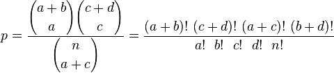
where  is the binomial coefficient and the symbol ! indicates the factorial operator. With the data above, this gives
  0.001346076.
The formula above gives the exact hypergeometric probability of observing this particular arrangement of the data, assuming the given marginal totals, on the null hypothesis that men and women are equally likely to be dieters. To put it another way, if we assume that the probability that a man is a dieter is p, the probability that a woman is a dieter is p, and we assume that both men and women enter our sample independently of whether or not they are dieters, then this hypergeometric formula gives the conditional probability of observing the values a, b, c, d in the four cells, conditionally on the observed marginals (i.e., assuming the row and column totals shown in the margins of the table are given). This remains true even if men enter our sample with different probabilities than women. The requirement is merely that the two classification characteristics -- gender, and dieter (or not) -- are not associated.
For example, suppose we knew probabilities P,Q,p,q with P+Q=p+q=1 such that (male dieter, male non-dieter, female dieter, female non-dieter) had respective probabilities (Pp,Pq,Qp,Qq) for each individual encountered under our sampling procedure. Then still, were we to calculate the distribution of cell entries conditional given marginals, we would obtain the above formula in which neither p nor P occurs. Thus, we can calculate the exact probability of any arrangement of the 24 teenagers into the four cells of the table, but Fisher showed that to generate a significance level, we need consider only the cases where the marginal totals are the same as in the observed table, and among those, only the cases where the arrangement is as extreme as the observed arrangement, or more so. (Barnard's test relaxes this constraint on one set of the marginal totals.) In the example, there are 11 such cases. Of these only one is more extreme in the same direction as our data; it looks like this:
| Men | Women | Row Total | |
|---|---|---|---|
| Dieting | 0 | 10 | 10 |
| Non-dieting | 12 | 2 | 14 |
| Column Total | 12 | 12 | 24 |
For this table (with extremely unequal dieting proportions) the probability is 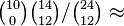 0.000033652.
In order to calculate the significance of the observed data, i.e. the total probability of observing data as extreme or more extreme if the null hypothesis is true, we have to calculate the values of p for both these tables, and add them together. This gives a one-tailed test, with p approximately 0.001346076 + 0.000033652 = 0.001379728. (For example, in the R statistical computing environment, this value can be obtained as fisher.test(rbind(c(1,9),c(11,3)), alternative="less")$p.value.) This value can be interpreted as the sum of evidence provided by the observed data -- or any more extreme table -- for the null hypothesis (that there is no difference in the proportions of dieters between men and women). The smaller the value of p, the greater the evidence for rejecting the null hypothesis; so here the evidence is strong that men and women are not equally likely to be dieters.
For a two-tailed test we must also consider tables that are equally extreme, but in the opposite direction. Unfortunately, classification of the tables according to whether or not they are 'as extreme' is problematic. An approach used by the fisher.test function in R is to compute the p-value by summing the probabilities for all tables with probabilities less than or equal to that of the observed table. In the example here, the 2-sided p-value is twice the 1-sided value -- but In general these can differ substantially for tables with small counts, unlike the case with test statistics that have a symmetric sampling distribution.
As noted above, most modern statistical packages will calculate the significance of Fisher tests, in some cases even where the chi-squared approximation would also be acceptable. The actual computations as performed by statistical software packages will as a rule differ from those described above, because numerical difficulties may result from the large values taken by the factorials. A simple, somewhat better computational approach relies on a gamma function or log-gamma function, but methods for accurate computation of hypergeometric and binomial probabilities remains an active research area.
Despite the fact that Fisher's test gives exact p-values, some authors have argued that it is conservative, i.e. that its actual rejection rate is below the nominal significance level.[10][11][12] The apparent contradiction stems from the combination of a discrete statistic with fixed significance levels.[13][14] To be more precise, consider the following proposal for a significance test at the 5%-level: reject the null hypothesis for each table to which Fisher's test assigns a p-value equal to or smaller than 5%. Because the set of all tables is discrete, there may not be a table for which equality is achieved. If  is the largest p-value smaller than 5% which can actually occur for some table, then the proposed test effectively tests at the -level. For small sample sizes, might be significantly lower than 5%.[10][11][12] While this effect occurs for any discrete statistic (not just in contingency tables, or for Fisher's test), it has been argued that the problem is compounded by the fact that Fisher's test conditions on the marginals.[15] To avoid the problem, many authors discourage the use of fixed significance levels when dealing with discrete problems.[13][14]
Another early discussion revolved around the necessity to condition on the marginals.[16][17] Fisher's test gives exact p-values both for fixed and for random marginals. Other tests, most prominently Barnard's, require random marginals. Some authors[13][14][17] (including, later, Barnard himself[13]) have criticized Barnard's test based on this property. They argue that the marginal totals are an (almost[14]) ancillary statistic, containing (almost) no information about the tested property.
An alternative exact test, Barnard's exact test, has been developed and proponents of it suggest that this method is more powerful, particularly in 2 × 2 tables. Another alternative is to use maximum likelihood estimates to calculate a p-value from the exact binomial or multinomial distributions and accept or reject based on the p-value.


 京公网安备 11010802025824号